Welcome to the next installment of our SQL journey! In our previous posts, we laid the groundwork for understanding databases and explored the setup of MSSQL. Now, it’s time to roll up our sleeves and dive into practical SQL commands. In this post, you’ll build a strong SQL foundation: you’ll learn about database and table creation, understand relational structures that prevent data duplication, and get hands-on with single-table queries, filtering, grouping, and key constraints—all using a realistic business scenario you’ll build on in the next parts.
We’ll be using a simulated e-commerce scenario to illustrate these concepts, transforming our database, tables, and column names into easily understandable examples.
Now, you can start your SSMS (Client) and connect it to the MSSQL Server installed earlier in order to practice what we are going to explore in this blog!
Let’s start with a Database first!
Setting Up Your Database: CREATE DATABASE and USE
Before we can store any data, we need a place for it to reside – a database!
CREATE DATABASE
- Purpose: This command, part of Data Definition Language (DDL), creates a brand new database. It defines the structure of your database before you add any data.
- Syntax:
CREATE DATABASE database_name;- Example: Let’s create an
eCommercedatabase to manage our online store’s data.
-- Create the eCommerce database
CREATE DATABASE eCommerce;- Expected Result: A new database named
eCommercewill be created on your SQL Server instance. You won’t see a visible output in the query window, but it will appear in your database list in SSMS’s Object Explorer.
USE
- Purpose: After creating a database, you need to tell SQL Server which database you intend to work with. The
USEcommand sets the active database context for subsequent queries. - Syntax:
USE database_name;- Example:
-- Select the eCommerce database to work within
USE eCommerce;Expected Result: The context in your SQL Server Management Studio (SSMS) query window will change to eCommerce, or subsequent queries will execute against this database.
Building Your Tables: CREATE TABLE, Data Types, and Constraints
Tables are the fundamental structures within a database where your data is organized into rows and columns. They are the blueprint for how your data will be stored, and defining them correctly is crucial for data integrity and efficiency.
CREATE TABLE
- Purpose: This DDL command defines a new table, including its columns, their respective data types, and constraints like primary keys.
- Syntax:
CREATE TABLE table_name (
    column1_name DataType NULL/NOT NULL,
    column2_name DataType NULL/NOT NULL,
    ...,
    [CONSTRAINT definitions for PK, FK, etc.]
);Understanding Data Types: The Building Blocks of Columns
Data types tell the database what kind of information a column will hold (e.g., numbers, text, dates) and how much space to allocate for it. SQL Server (and other SQL databases) offers a rich variety of data types. Here are some common ones:
INT: Stores whole numbers (integers). Ideal for IDs, counts, or quantities.VARCHAR(size): Stores variable-length non-Unicode string data. Thesizespecifies the maximum number of characters. Perfect for names, cities, or short descriptions.NVARCHAR(size): Similar toVARCHARbut stores variable-length Unicode string data. Use this when you need to store characters from multiple languages (e.g., English, Chinese, Arabic).TEXT/NTEXT: For very large string data.NTEXTsupports Unicode. (Note:VARCHAR(MAX)/NVARCHAR(MAX)are generally preferred overTEXT/NTEXTin modern SQL Server versions).DECIMAL(precision, scale): Stores numbers with a fixed precision and scale.precisionis the total number of digits (before and after the decimal), andscaleis the number of digits after the decimal point. Useful for currency or percentages where exact values are crucial.FLOAT/REAL: Stores approximate floating-point numbers. Use these for scientific calculations where precision isn’t paramount, but range is important.DATE: Stores dates only (YYYY-MM-DD).TIME: Stores time only (HH:MM:SS.nnnnnnn).DATETIME/DATETIME2: Stores both date and time.DATETIME2offers greater precision and range.BIT: Stores boolean values (0 for false, 1 for true). Ideal for flags or yes/no indicators.
Column Constraints: Defining Data Rules
Constraints enforce rules on the data in a table, ensuring data integrity and consistency.
NOT NULL: This is a column constraint explicitly stated to ensure that the column cannot containNULL(empty) values. This means data must be provided for this column every time a new row is inserted.NULL(Default Behavior): If you do not explicitly specifyNOT NULLfor a column, the default behavior in SQL (and specifically SQL Server) is to allowNULLvalues. This means you can leave that column empty when inserting or updating records, and it will storeNULL. It’s good practice to explicitly defineNULLif that’s your intention for clarity, though it’s not strictly required by the parser.
Key Constraints: Linking and Identifying Data
Keys are a special type of constraint that define relationships between tables and ensure unique identification of records.
PRIMARY KEY(PK):- Purpose: A crucial constraint that uniquely identifies each row in a table. Think of it as the table’s unique ID badge.
- Characteristics:
- It cannot contain
NULLvalues. - It must contain unique values for each row.
- Every table should ideally have one primary key.
- It cannot contain
FOREIGN KEY(FK):- Purpose: A constraint that links two tables together by referencing the
PRIMARY KEYof another table. It enforces referential integrity, ensuring that relationships between tables are maintained and valid. - Example: In an e-commerce system, a
client_idin anOrderstable might be aFOREIGN KEYreferencing theclient_id(which is aPRIMARY KEY) in aClientAccountstable. This ensures that every order is associated with a valid, existing client.
- Purpose: A constraint that links two tables together by referencing the
Example 1:
- Creating
TeamMembersTable.- Let’s create a table for our e-commerce team members, including their ID, name, location, and commission rate. All these fields are essential, so we mark them
NOT NULL.
- Let’s create a table for our e-commerce team members, including their ID, name, location, and commission rate. All these fields are essential, so we mark them
-- Create the TeamMembers table
CREATE TABLE TeamMembers (
    member_id INT NOT NULL,
    member_name VARCHAR(50) NOT NULL,
    location_city VARCHAR(50) NOT NULL,
    commission_rate DECIMAL(4,2) NOT NULL,
    PRIMARY KEY (member_id) -- member_id is the unique identifier for each team member
);- Expected Result: After running below query, an empty table named
TeamMemberswill be created in youreCommercedatabase.
Example 2:
- Creating
ClientAccountsTable with a Foreign Key.- Next, we’ll create a table for our clients, linking them to a
TeamMemberwho is assigned to serve them. This demonstrates the use of aFOREIGN KEY.
- Next, we’ll create a table for our clients, linking them to a
-- Create the ClientAccounts table
CREATE TABLE ClientAccounts (
    client_id INT NOT NULL,
    client_name VARCHAR(50) NOT NULL,
    client_city VARCHAR(50) NOT NULL,
    satisfaction_rating INT NOT NULL,
    assigned_member_id INT NOT NULL,
    PRIMARY KEY (client_id), -- client_id is the unique identifier for each client
    FOREIGN KEY (assigned_member_id) REFERENCES TeamMembers(member_id) -- Links to TeamMembers table
);- Expected Result: An empty
ClientAccountstable is created. Theassigned_member_idcolumn is now constrained to only acceptmember_idvalues that already exist in theTeamMemberstable.
Example 3:
- Creating a
LearnersTable.- This table further illustrates the difference between
NULLandNOT NULLconstraints. Notice howlearner_cityis explicitly defined asNULL(or could be omitted for the same default behavior).
- This table further illustrates the difference between
CREATE TABLE Learners (
    learner_id INT NOT NULL,
    learner_name VARCHAR(50) NOT NULL,
    learner_city VARCHAR(50) NULL, -- This column can explicitly be empty (NULL)
    zip_code VARCHAR(10) NOT NULL,
    PRIMARY KEY (learner_id)
);- Expected Result: An empty
Learnerstable is created. When inserting data, you can choose to leavelearner_cityblank (it will storeNULL), while otherNOT NULLcolumns must always have a value.
Inspecting Table Structure: EXEC sp_help
Before inserting data or if you need a reminder of a table’s design, you can quickly review its structure.
EXEC sp_help
- Purpose: This is a SQL Server-specific stored procedure that provides detailed information about a database object, such as a table. This includes its columns, data types, nullability, constraints, and indexes. It’s a quick way to get a schema overview.
- Syntax:
EXEC sp_help table_name;- Example:
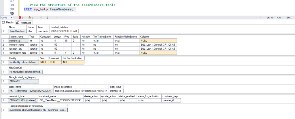
-- View the structure of the TeamMembers table
EXEC sp_help TeamMembers;- Expected Result: A detailed report will appear in your results pane showing column names, their data types, whether they allow nulls, and other properties of the
TeamMemberstable.
Adding Data to Tables: INSERT INTO
Once your tables are defined, you can populate them with actual records. This is where the data comes to life!
INSERT INTO (Single Row)
- Purpose: This Data Manipulation Language (DML) command adds a single new row (record) into a table.
- Syntax:
INSERT INTO table_name VALUES (value1, value2, ...);
-- Or, to insert into specific columns:
INSERT INTO table_name (column1, column2) VALUES (value1, value2);- Example:
-- Insert a single record for a team member
INSERT INTO TeamMembers VALUES (101, 'Alice Smith', 'London', 0.12);- Expected Result: One new row will be added to the
TeamMemberstable.
INSERT INTO (Multiple Rows in One Statement)
- Purpose: You can efficiently insert several rows into a table using a single
INSERTstatement by separating the sets of values for each row with commas. - Syntax:
INSERT INTO table_name VALUES (value1_row1, ...), (value1_row2, ...), ...;- Examples:
-- Insert additional team members, one at a time for demonstration
INSERT INTO TeamMembers VALUES (102, 'Bob Johnson', 'San Jose', 0.13);
INSERT INTO TeamMembers VALUES (104, 'Charlie Brown', 'London', 0.11);

-- Insert multiple team members at once
INSERT INTO TeamMembers VALUES
    (107, 'David Lee', 'Barcelona', 0.15),
    (103, 'Eve Davis', 'New York', 0.10),
    (105, 'Fran White', 'London', 0.26);

-- Insert records into ClientAccounts
INSERT INTO ClientAccounts VALUES (2001, 'Hoffman Corp', 'London', 100, 101);
INSERT INTO ClientAccounts VALUES
    (2002, 'Giovanni Ltd', 'Rome', 200, 103),
    (2003, 'Liu Enterprises', 'San Jose', 200, 102),
    (2004, 'Grass Solutions', 'Berlin', 300, 102),
    (2006, 'Clemens Inc', 'London', 100, 101),
    (2008, 'Cisneros Group', 'San Jose', 300, 107),
    (2007, 'Pereira Services', 'Rome', 100, 104);

-- Insert into Learners, demonstrating how to omit a NULLable column
INSERT INTO Learners (learner_id, learner_name, zip_code) VALUES (1, 'John Doe', '12345');
- Expected Result: Each
INSERTstatement will successfully add the specified number of rows to its respective table.
Retrieving Data: SELECT and Filtering with WHERE
The SELECT statement is arguably the most frequently used SQL command. It allows you to retrieve data from your tables, and the WHERE clause empowers you to refine your results.
SELECT *
- Purpose: Retrieves all columns from a specified table. The
*acts as a wildcard, meaning “all columns.” - Syntax:]
SELECT * FROM table_name;- Example:
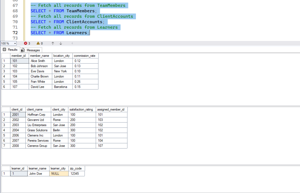
-- Fetch all records from TeamMembers
SELECT * FROM TeamMembers;
-- Fetch all records from ClientAccounts
SELECT * FROM ClientAccounts;
-- Fetch all records from Learners
SELECT * FROM Learners;- Expected Result: All rows and all columns from the specified table will be displayed in the results pane.
SELECT with Specific Columns
- Purpose: To retrieve only a subset of columns, you list their names explicitly instead of using
*. This is good practice for performance and clarity. - Syntax:
SELECT column1, column2 FROM table_name;- Example:
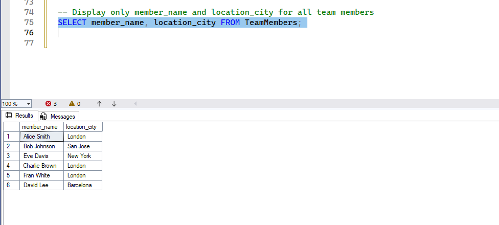
-- Display only member_name and location_city for all team members
SELECT member_name, location_city FROM TeamMembers;- Expected Result: Only the
member_nameandlocation_citycolumns will be shown for all rows in theTeamMemberstable.
Filtering with WHERE Clause
The WHERE clause is essential for filtering records based on specific conditions, helping you find exactly the data you need.
- Using
=(Equality)- Purpose: To find records where a column’s value exactly matches a specified value.Example:
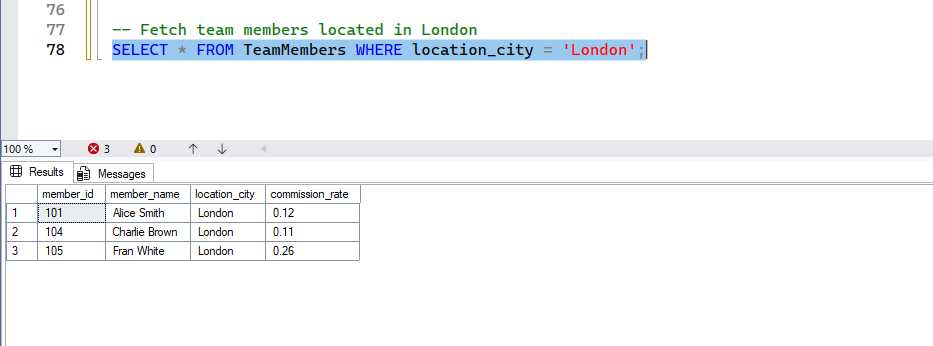
-- Fetch team members located in London
SELECT * FROM TeamMembers WHERE location_city = 'London';- Expected Result: Only rows where
location_cityis ‘London’ will be displayed.
- Using
OR(Logical OR)- Purpose: To find records that satisfy at least one of several conditions. If any condition after
ORis true, the row is included.
- Purpose: To find records that satisfy at least one of several conditions. If any condition after
- Example:
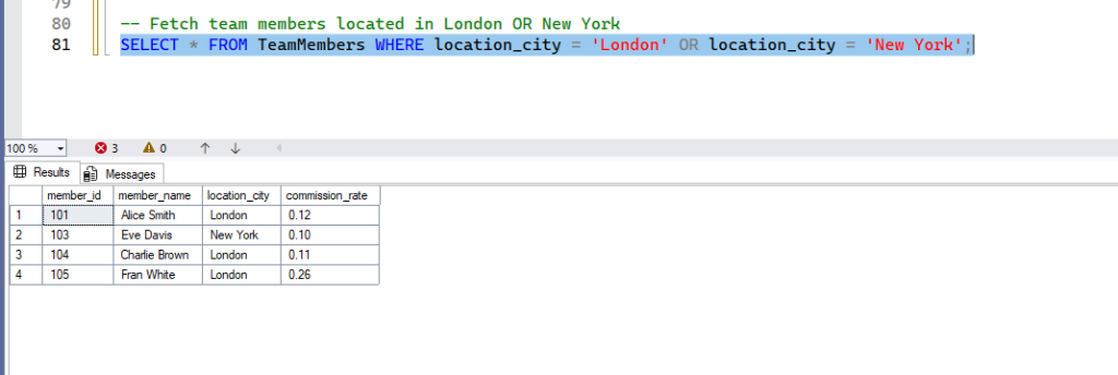
-- Fetch team members located in London OR New York
SELECT * FROM TeamMembers WHERE location_city = 'London' OR location_city = 'New York';- Expected Result: Rows where
location_cityis either ‘London’ or ‘New York’ will be displayed.
- Using
IN(List of Values)- Purpose: A concise shorthand for multiple
ORconditions, useful when checking if a column’s value is within a specified list of values.
- Purpose: A concise shorthand for multiple
- Example:
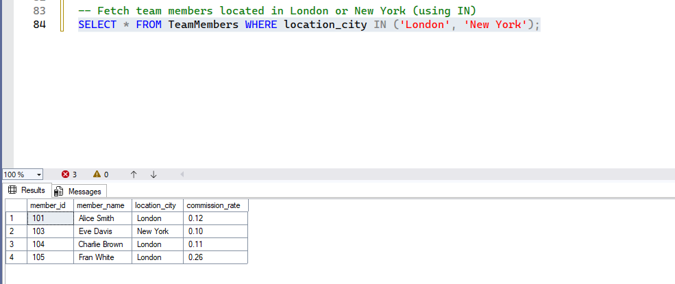
-- Fetch team members located in London or New York (using IN)
SELECT * FROM TeamMembers WHERE location_city IN ('London', 'New York');- Expected Result: Same as above OR
- Using
>=and<=(Range withAND)- Purpose: To find records where a numeric or date value falls within a specified range. The
ANDoperator requires both conditions to be true for a row to be included.
- Purpose: To find records where a numeric or date value falls within a specified range. The
- Example:
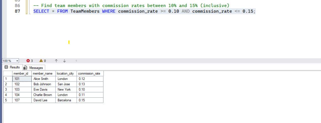
-- Find team members with commission rates between 10% and 15% (inclusive)
SELECT * FROM TeamMembers WHERE commission_rate >= 0.10 AND commission_rate <= 0.15;- Expected Result: Only team members with commission rates from 0.10 to 0.15 will be shown.

- Using
BETWEEN(Range Shorthand)- Purpose: A more readable and concise way to specify a range for numeric or date values. It’s inclusive of the start and end values.
- Example:
-- Find team members with commission rates between 10% and 15% (using BETWEEN)
SELECT * FROM TeamMembers WHERE commission_rate BETWEEN 0.10 AND 0.15;- Expected Result: TeamMembers having commission rate in given condition will be fetched.
- Combining
ANDwith other operators:- Purpose: To apply multiple filtering conditions where all conditions must be true for a row to be included.
- Example:
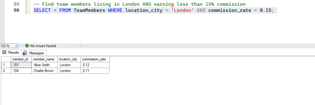
-- Find team members living in London AND earning less than 15% commission
SELECT * FROM TeamMembers WHERE location_city = 'London' AND commission_rate < 0.15; - Expected Result: Only London-based team members with a commission rate strictly less than 0.15 will appear.
- Complex
WHEREconditions (combiningANDandOR)- Purpose: To create more sophisticated filters using parentheses to define the order of operations, just like in math.Example:
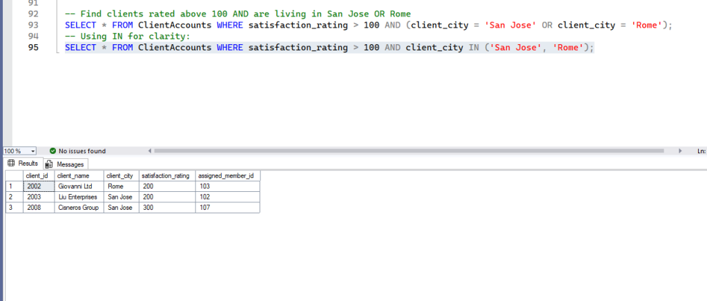
-- Find clients rated above 100 AND are living in San Jose OR Rome
SELECT * FROM ClientAccounts WHERE satisfaction_rating > 100 AND (client_city = 'San Jose' OR client_city = 'Rome');
-- Using IN for clarity:
SELECT * FROM ClientAccounts WHERE satisfaction_rating > 100 AND client_city IN ('San Jose', 'Rome');Expected Result: Bothe the query will have the same result as below.
The LIKE Operator: Your Gateway to Pattern Matching
The LIKE operator is used in the WHERE clause of a SELECT, INSERT, UPDATE, or DELETE statement to search for a specified pattern in a column. It’s almost always used with wildcard characters, which represent one or more characters.
Basic Syntax:
SELECT column1, column2
FROM table_name
WHERE column_name LIKE 'pattern';Wildcard Characters in MSSQL
MSSQL provides several wildcard characters that you can combine to create powerful search patterns:
%(Percentage Sign): Represents zero, one, or multiple characters.- Think of it as a flexible placeholder for any sequence of characters.
_(Underscore): Represents a single character.- Think of it as a fixed placeholder for exactly one character.
[](Square Brackets): Represents any single character within the specified set.- Example:
[abc]matches ‘a’, ‘b’, or ‘c’. - Example:
[a-f]matches any character from ‘a’ through ‘f’.
- Example:
[^](Caret within Square Brackets): Represents any single character not within the specified set.- Example:
[^abc]matches any character except ‘a’, ‘b’, or ‘c’. - Example:
[^a-f]matches any character not from ‘a’ through ‘f’.
- Example:
Let’s dive into examples!
Examples Using % (Zero or More Characters)
The % wildcard is incredibly versatile for finding values that start with, end with, or contain a specific sequence.
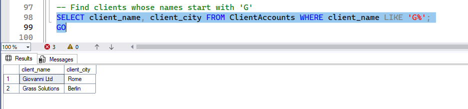
-- Find clients whose names start with 'G'
SELECT client_name, client_city FROM ClientAccounts WHERE client_name LIKE 'G%';
GO

-- Find team members whose names end with 'son'
SELECT member_name, location_city FROM TeamMembers WHERE member_name LIKE '%son';
GO

-- Find clients whose city contains 'on' (e.g., London, San Jose)
SELECT client_name, client_city FROM ClientAccounts WHERE client_city LIKE '%on%';
GO

-- Find client names that contain 'Inc' (e.g., 'Tech Solutions Inc.')
SELECT client_name FROM ClientAccounts WHERE client_name LIKE '%Inc%';
GO

-- Find clients whose names do NOT contain 'Corp'
SELECT client_name FROM ClientAccounts WHERE client_name NOT LIKE '%Corp%';
GO- Expected Result: Run the queries one by one and see the result. Here is the output for the first one.
Examples Using _ (Exactly One Character)
The _ wildcard is useful when you know the exact length of a part of the string or a character’s position.
-- Find team members whose name has 'o' as the second letter (e.g., Bob Johnson)
SELECT member_name FROM TeamMembers WHERE member_name LIKE '_o%';
GO

-- Find client names that are exactly 12 characters long (e.g., 'Clemens Inc')
SELECT client_name FROM ClientAccounts WHERE client_name LIKE '____________';
GO

-- Find cities that are exactly 6 characters long (e.g., 'London', 'Berlin', 'New York' would not match)
SELECT DISTINCT location_city FROM TeamMembers WHERE location_city LIKE '______';
GOExamples Using [] (Any Single Character in a Set)
This wildcard allows you to specify a range or a list of characters for a single position.
-- Find clients whose name starts with 'G' or 'L'
SELECT client_name FROM ClientAccounts WHERE client_name LIKE '[GL]%';
GO

-- Find team members whose name starts with any letter from 'A' to 'C'
SELECT member_name FROM TeamMembers WHERE member_name LIKE '[A-C]%';
GO

-- Find client cities that start with 'R' or 'B' (e.g., Rome, Berlin)
SELECT client_city FROM ClientAccounts WHERE client_city LIKE '[RB]%';
GOExamples Using [^] (Any Single Character NOT in a Set)
The [^] wildcard is the inverse of [], matching any character not within the specified set.
-- Find clients whose name does NOT start with 'G' or 'L'
SELECT client_name FROM ClientAccounts WHERE client_name LIKE '[^GL]%';
GO

-- Find team members whose name does NOT start with any letter from 'A' to 'C'
SELECT member_name FROM TeamMembers WHERE member_name LIKE '[^A-C]%';
GO

-- Find client cities that do NOT start with 'R' or 'B'
SELECT client_city FROM ClientAccounts WHERE client_city LIKE '[^RB]%';
GOCombining Wildcards for Complex Patterns
You can combine these wildcards to create very specific search patterns.
-- Find client names that start with 'H', have 'o' as the second character, and end with 'Corp'
-- (e.g., 'Hoffman Corp')
SELECT client_name FROM ClientAccounts WHERE client_name LIKE 'Ho%Corp';
GO

-- Find team members whose city starts with 'L' and has 'n' as the third character,
-- and is exactly 6 characters long (e.g., 'London')
SELECT member_name, location_city FROM TeamMembers WHERE location_city LIKE 'L_n___';
GO

-- Find client names that start with 'C', followed by any character, then 'e', and end with 's Inc'
-- (e.g., 'Clemens Inc')
SELECT client_name FROM ClientAccounts WHERE client_name LIKE 'C_e%s Inc';
GOEscaping Wildcard Characters
What if your data actually contains a % or _ character, and you want to search for that literal character instead of treating it as a wildcard? You use the ESCAPE clause.
The ESCAPE clause allows you to define an escape character. Any character immediately following the escape character in the pattern string will be interpreted as a literal character rather than a wildcard.
Syntax:
WHERE column_name LIKE 'pattern' ESCAPE 'escape_character';Example: Imagine a client name like Client_A%B. If you search LIKE 'Client_A%', it will match Client_A_ or Client_ABC. To find Client_A%B literally, you need to escape the %.
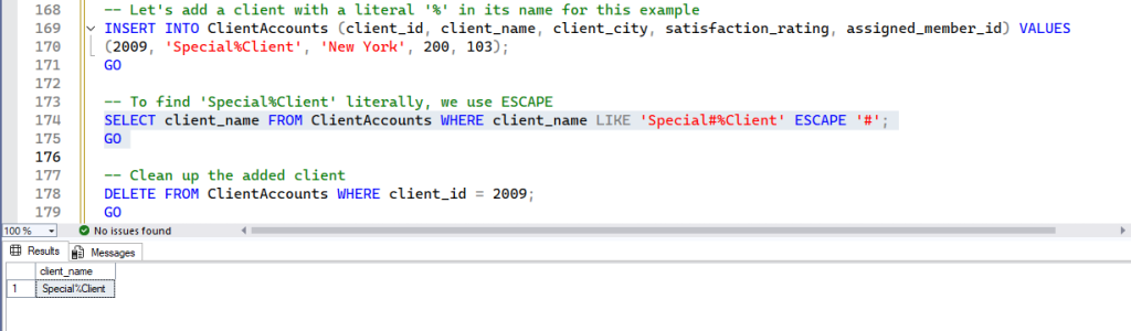
-- Let's add a client with a literal '%' in its name for this example
INSERT INTO ClientAccounts (client_id, client_name, client_city, satisfaction_rating, assigned_member_id) VALUES
(2009, 'Special%Client', 'New York', 200, 103);
GO

-- To find 'Special%Client' literally, we use ESCAPE
SELECT client_name FROM ClientAccounts WHERE client_name LIKE 'Special#%Client' ESCAPE '#';
GO

-- Clean up the added client
DELETE FROM ClientAccounts WHERE client_id = 2009;
GOHow it works: We defined # as our escape character. When LIKE sees #%, it knows to treat the % as a literal character, not a wildcard. You can choose any character as your escape character, as long as it’s not a wildcard itself and doesn’t appear unescaped in your actual pattern.
Pattern matching with the LIKE operator and its versatile wildcard characters (%, _, [], [^]) is an indispensable skill for any SQL developer. It allows you to perform flexible and powerful searches on string data, going beyond simple equality checks. By combining these wildcards, you can construct highly specific patterns to extract exactly the data you need. Remember to use the ESCAPE clause when you need to search for literal wildcard characters within your data.
Aggregating Data: COUNT and GROUP BY
SQL provides powerful aggregate functions to perform calculations on sets of rows, rather than individual rows.
COUNT(*) and COUNT(column)
- Purpose:
COUNT(*): Counts all rows in a table (including rows where some columns might haveNULLvalues).COUNT(column_name): Counts only the non-NULLvalues in a specific column.
- Syntax:
SELECT COUNT(*) FROM table_name;

SELECT COUNT(column_name) AS 'Alias Name' FROM table_name;- Examples:
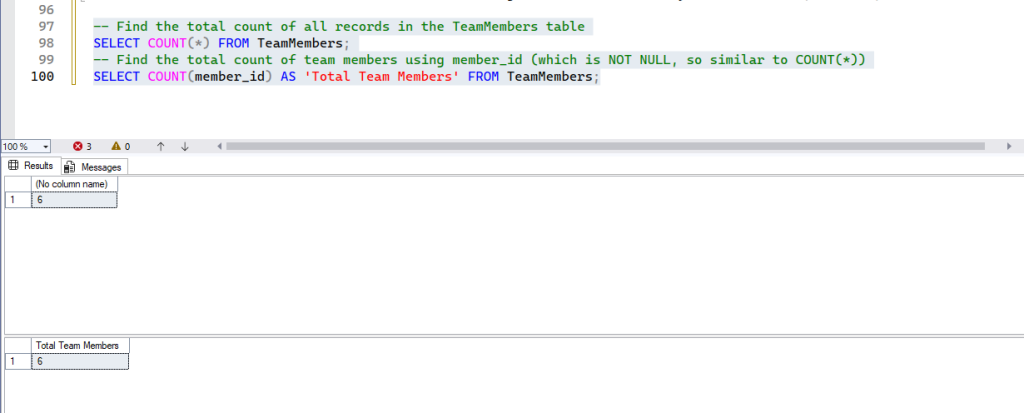
-- Find the total count of all records in the TeamMembers table
SELECT COUNT(*) FROM TeamMembers;
-- Find the total count of team members using member_id (which is NOT NULL, so similar to COUNT(*))
SELECT COUNT(member_id) AS 'Total Team Members' FROM TeamMembers;- Expected Result: A single number representing the total count of rows or non-null values for the specified column. Run both the queries in one go and you will see the result like below.
GROUP BY
- Purpose: This clause is typically used with aggregate functions (like
COUNT,SUM,AVG,MIN,MAX). It organizes rows that have the same values in specified columns into a summary row for each group. This allows you to perform calculations per category. - Syntax:
SELECT column_to_group_by, AGGREGATE_FUNCTION(column_to_aggregate)
FROM table_name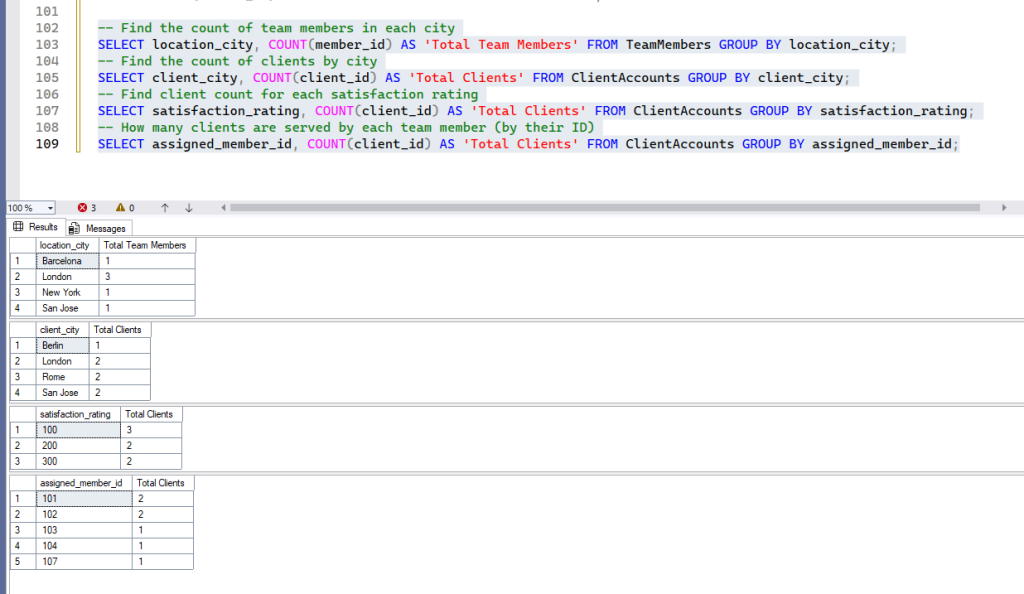
GROUP BY column_to_group_by;- Examples:
-- Find the count of team members in each city
SELECT location_city, COUNT(member_id) AS 'Total Team Members' FROM TeamMembers GROUP BY location_city;
-- Find the count of clients by city
SELECT client_city, COUNT(client_id) AS 'Total Clients' FROM ClientAccounts GROUP BY client_city;
-- Find client count for each satisfaction rating
SELECT satisfaction_rating, COUNT(client_id) AS 'Total Clients' FROM ClientAccounts GROUP BY satisfaction_rating;
-- How many clients are served by each team member (by their ID)
SELECT assigned_member_id, COUNT(client_id) AS 'Total Clients' FROM ClientAccounts GROUP BY assigned_member_id;- Expected Result: A result set showing each unique city (or rating, or assigned member ID) and the corresponding count of records for that group. Run queries one by one to see the result, or in one go. Here is the result after running all above queries in one go.
Sorting Data: ORDER BY
The ORDER BY clause is used to sort the result set of a SELECT query based on one or more columns.
ORDER BY (ASC and DESC)
- Purpose: Arranges the output in ascending (
ASC, which is the default, so it can be omitted) or descending (DESC) order based on one or more specified columns. - Syntax:
SELECT columns FROM table_name ORDER BY column_to_sort ASC/DESC;- Examples:
-- Arrange TeamMembers output in ascending order of member_name
SELECT member_name, location_city FROM TeamMembers ORDER BY member_name;
-- Explicitly ascending (same result as above)
SELECT member_name, location_city FROM TeamMembers ORDER BY member_name ASC;
-- Descending order of member_name
SELECT member_name, location_city FROM TeamMembers ORDER BY member_name DESC;
-- Arrange client table by client_city
SELECT * FROM ClientAccounts ORDER BY client_city;
-- Find count of clients by city for London and New York, then order by ascending count
SELECT client_city, COUNT(client_id) AS 'Count of Clients'
FROM ClientAccounts
WHERE client_city IN ('London', 'New York')
GROUP BY client_city
ORDER BY COUNT(client_id) ASC;
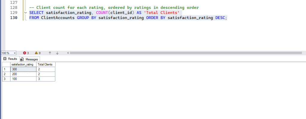
-- Client count for each rating, ordered by ratings in descending order
SELECT satisfaction_rating, COUNT(client_id) AS 'Total Clients'
FROM ClientAccounts GROUP BY satisfaction_rating ORDER BY satisfaction_rating DESC;- Expected Result: The rows in the result set will be sorted according to the specified column and order. Run the queries one by one to see the result. Here is the output of the last one – Client count for each rating, ordered by ratings in descending order.
Filtering Groups: The Power of SQL’s HAVING Clause
We learnt how to group data using GROUP BY and how to sort results with ORDER BY. We also learned to filter individual rows using the WHERE clause. Now, imagine you have grouped your data and performed calculations like counting or averaging. What if you need to filter these groups themselves based on the aggregated results? This is precisely where the HAVING clause becomes indispensable.
The HAVING clause acts like a WHERE clause, but it specifically targets and filters the results of a GROUP BY operation. It allows you to apply conditions to aggregated data, such as COUNT(), SUM(), AVG(), MAX(), or MIN()., don’t worry for this functions for now, we are going to learn them in detail while covering Functions.
Why Can’t WHERE Do This?
It’s a common question: “Why not just use WHERE?” The answer lies in the order of operations within SQL. The WHERE clause processes individual rows before any grouping or aggregation takes place. Therefore, you cannot use aggregate functions directly within a WHERE clause.
The HAVING clause, on the other hand, operates after the GROUP BY clause has created the groups and the aggregate functions have calculated their values for each group. This sequential processing makes HAVING the perfect tool for filtering summarized data.
Syntax:
The HAVING clause always follows the GROUP BY clause in a SQL query.
SELECT
    column1,
    aggregate_function(column2)
FROM
    TableName
WHERE
    condition_on_individual_rows -- (Optional) Filters rows before grouping
GROUP BY
    column1
HAVING
condition_on_groups; -- Filters groups based on aggregate resultsKey takeaways for HAVING:
- It is used after
GROUP BY. - It filters results of aggregate functions.
- It operates on groups, not individual rows.
Practical Examples:
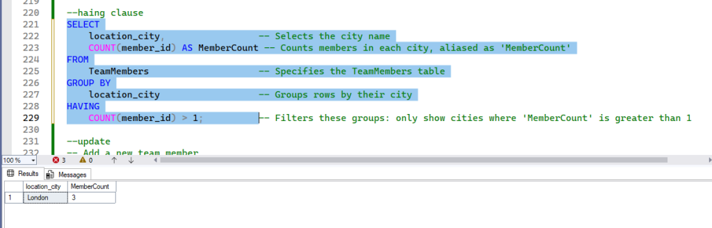
Example 1: Identifying Cities with Multiple Team Members
Let’s find all location_city entries that have more than one TeamMember assigned.
SELECT
    location_city,                 -- Selects the city name
    COUNT(member_id) AS MemberCount -- Counts members in each city, aliased as 'MemberCount'
FROM
    TeamMembers                    -- Specifies the TeamMembers table
GROUP BY
    location_city                  -- Groups rows by their city
HAVING
COUNT(member_id) > 1; -- Filters these groups: only show cities where 'MemberCount' is greater than 1How it works:
- The query first groups all
TeamMembersby theirlocation_city. - Then, for each city,
COUNT(member_id)calculates the total number of team members. - Finally,
HAVING COUNT(member_id) > 1filters these summarized city groups, keeping only those that have aMemberCountgreater than 1.
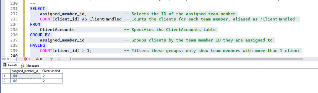
Example 2: Finding Team Members Managing More Than One Client
We want to know which assigned_member_id (team members) are handling more than one ClientAccount.
SELECT
    assigned_member_id,               -- Selects the ID of the assigned team member
    COUNT(client_id) AS ClientHandled -- Counts the clients for each team member, aliased as 'ClientHandled'
FROM
    ClientAccounts                    -- Specifies the ClientAccounts table
GROUP BY
    assigned_member_id                -- Groups clients by the team member ID they are assigned to
HAVING
COUNT(client_id) > 1; -- Filters these groups: only show team members with more than 1 clientHow it works:
- The query groups records in
ClientAccountsbyassigned_member_id. COUNT(client_id)determines how many clients eachassigned_member_idhas.HAVING COUNT(client_id) > 1then filters these groups, showing only those team members who manage more than one client.
Modifying Existing Data: UPDATE
UPDATE
- Purpose: This DML command is used to modify existing records (rows) in a table. It’s crucial to use the
WHEREclause withUPDATEto specify which rows to modify; without aWHEREclause, all rows in the table will be updated! - Syntax:
UPDATE table_name
SET column1 = new_value1, column2 = new_value2, ...
WHERE condition;- Examples: First, let’s add a temporary team member for demonstration purposes:
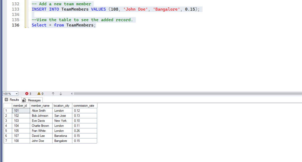
-- Add a new team member
INSERT INTO TeamMembers VALUES (108, 'John Doe', 'Bangalore', 0.15);

--View the table to see the added record.
Select * from TeamMembers;Execute this to see the below result:
Now, let’s perform updates:
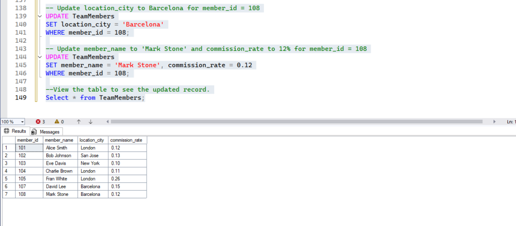
-- Update location_city to Barcelona for member_id = 108
UPDATE TeamMembers
SET location_city = 'Barcelona'
WHERE member_id = 108;

-- Update member_name to 'Mark Stone' and commission_rate to 12% for member_id = 108
UPDATE TeamMembers
SET member_name = 'Mark Stone', commission_rate = 0.12
WHERE member_id = 108;

--View the table to see the updated record.
Select * from TeamMembers;- Expected Result: The specified column(s) in the row(s) matching the
WHEREcondition will be changed as shown below –
Deleting Data: DELETE FROM
DELETE FROM
- Purpose: This DML command removes existing rows from a table. Like
UPDATE, theWHEREclause is essential to specify which rows to delete; without it, all rows will be permanently removed from the table! - Syntax:
DELETE FROM table_name WHERE condition;- Example:
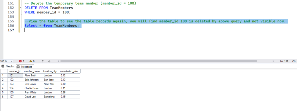
-- Delete the temporary team member (member_id = 108)
DELETE FROM TeamMembers
WHERE member_id = 108;- Expected Result: The row(s) matching the
WHEREcondition will be permanently removed from the table.
Exploring Unique Values: DISTINCT
DISTINCT
- Purpose: Used with the
SELECTstatement,DISTINCTreturns only unique (non-duplicate) values from a specified column or set of columns. It’s great for quickly seeing all the different categories within a column. - Syntax:
SELECT DISTINCT column_name FROM table_name;- Examples:
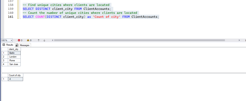
-- Find unique cities where clients are located
SELECT DISTINCT client_city FROM ClientAccounts;
-- Count the number of unique cities where clients are located
SELECT COUNT(DISTINCT client_city) FROM ClientAccounts;- Expected Result: A list showing each unique city only once, or the total count of those unique cities.
Conclusion
You’ve now completed a hands-on tour of essential SQL commands for managing and querying data within a single table or identifying relationships between them! From defining your database structure with DDL (CREATE DATABASE, CREATE TABLE) to manipulating data with DML (INSERT, UPDATE, DELETE), and querying and analyzing data with DQL (SELECT, WHERE, PATTERN MATCHING GROUP BY, ORDER BY, HAVING, DISTINCT), you have a solid foundation.
These commands are the building blocks of almost any interaction with a relational database. Keep practicing, and you’ll soon be proficient in managing and extracting valuable insights from your data!
Stay tuned for our next blog post, where we’ll explore next concepts starting with SQL JOINs in more detail, learning how to effectively combine data from multiple related tables! Remember, we will build directly on these tables, introducing multi-table queries and SQL JOINs to answer bigger business questions. Make sure to save your demo data—you’ll use it again!
Leave a Reply
You must be logged in to post a comment.