Welcome back to our ongoing MSSQL series! In our previous post, we dived into Subqueries for precise data filtering and understood the foundational concept of Candidate Keys for robust database design.
Today, we’re expanding our toolkit even further by exploring three powerful features that enhance data presentation, analysis, and aggregation: Views (virtual tables for simplified data access), Ranking Window Functions (for assigning ranks within data sets), and the ROLLUP operator (for generating comprehensive summary reports). These tools are crucial for making your data more accessible, deriving insights, and creating flexible reports.
For this blog post, we will introduce entirely new datasets and table structures to demonstrate these concepts clearly, without relying on previous examples.
Setting Up Our Environment
To ensure you can follow along with all the examples, here are the table schemas and sample data we’ll be using. Please run the following scripts to set up your environment:
1. Table Creation Scripts
We will create new tables for our examples: Products, CustomerOrders, StudentScores, AthletePerformance, and EMPLOYEE.
-- Create the eCommerce database (if not created earlier)
CREATE DATABASE eCommerce;

-- Select the eCommerce database to work within
USE eCommerce;

-- Tables for Views Examples
CREATE TABLE Products (
    product_id INT NOT NULL PRIMARY KEY,
    product_name VARCHAR(100) NOT NULL,
    category VARCHAR(50) NOT NULL,
    unit_price DECIMAL(10, 2) NOT NULL,
    stock_quantity INT NOT NULL
);

CREATE TABLE CustomerOrders (
    order_id INT NOT NULL PRIMARY KEY,
    customer_name VARCHAR(100) NOT NULL,
    order_date DATE NOT NULL,
    product_id INT NOT NULL,
    quantity_ordered INT NOT NULL,
    total_amount DECIMAL(10, 2) NOT NULL,
    FOREIGN KEY (product_id) REFERENCES Products(product_id)
);
GO

-- Tables for Ranking Examples
CREATE TABLE StudentScores (
    student_id INT NOT NULL PRIMARY KEY,
    student_name VARCHAR(100) NOT NULL,
    subject VARCHAR(50) NOT NULL,
    score INT NOT NULL
);

CREATE TABLE AthletePerformance (
    athlete_id INT NOT NULL PRIMARY KEY,
    athlete_name VARCHAR(100) NOT NULL,
    event_name VARCHAR(50) NOT NULL,
    time_in_seconds DECIMAL(5, 2) NOT NULL
);
GO

-- Table for ROLLUP Example
CREATE TABLE EMPLOYEE (
    emp_id INT IDENTITY (1,1) PRIMARY KEY, -- IDENTITY (seed, increment) for auto-incrementing ID
    fullname VARCHAR(65),
    occupation VARCHAR(45),
    gender VARCHAR(30),
    salary INT,
    country VARCHAR(55)
);
GO
2. Inserting Sample Data
Let’s populate our new tables with some sample data.
-- Insert sample data into Products
INSERT INTO Products (product_id, product_name, category, unit_price, stock_quantity) VALUES
(1, 'Laptop Pro', 'Electronics', 1200.00, 50),
(2, 'Mechanical Keyboard', 'Accessories', 80.00, 200),
(3, 'Wireless Mouse', 'Accessories', 25.00, 300),
(4, '4K Monitor', 'Electronics', 450.00, 75),
(5, 'Gaming Headset', 'Audio', 100.00, 150);

-- Insert sample data into CustomerOrders
INSERT INTO CustomerOrders (order_id, customer_name, order_date, product_id, quantity_ordered, total_amount) VALUES
(101, 'Alice Wonderland', '2025-07-01', 1, 1, 1200.00),
(102, 'Bob The Builder', '2025-07-01', 2, 2, 160.00),
(103, 'Charlie Chaplin', '2025-07-02', 1, 1, 1200.00),
(104, 'Diana Prince', '2025-07-03', 4, 1, 450.00),
(105, 'Eve Harrington', '2025-07-03', 3, 3, 75.00),
(106, 'Frankenstein', '2025-07-04', 5, 1, 100.00),
(107, 'Grace Kelly', '2025-07-05', 1, 2, 2400.00),
(108, 'Harry Potter', '2025-07-05', 2, 1, 80.00),
(109, 'Ivy League', '2025-07-06', 4, 1, 450.00),
(110, 'Jack Sparrow', '2025-07-07', 3, 2, 50.00);

-- Insert sample data into StudentScores
INSERT INTO StudentScores (student_id, student_name, subject, score) VALUES
(1, 'Alice', 'Math', 95),
(2, 'Bob', 'Math', 88),
(3, 'Charlie', 'Math', 95),
(4, 'Diana', 'Science', 92),
(5, 'Eve', 'Science', 88),
(6, 'Frank', 'Science', 92),
(7, 'Grace', 'History', 78),
(8, 'Harry', 'History', 85);

-- Insert sample data into AthletePerformance
INSERT INTO AthletePerformance (athlete_id, athlete_name, event_name, time_in_seconds) VALUES
(101, 'Bolt', '100m Dash', 9.58),
(102, 'Powell', '100m Dash', 9.72),
(103, 'Gatlin', '100m Dash', 9.72),
(104, 'Wariner', '400m Run', 43.45),
(105, 'Merritt', '400m Run', 43.65),
(106, 'Johnson', '400m Run', 43.18),
(107, 'Gore', '100m Dash', 9.75),
(108, 'Warn', '400m Run', 43.45);

-- Insert sample data into EMPLOYEE
INSERT INTO EMPLOYEE(fullname, occupation, gender, salary, country) VALUES
('John Doe', 'Writer', 'Male', 62000, 'USA'),
('Mary Greenspan', 'Freelancer', 'Female', 55000, 'India'),
('Grace Smith', 'Scientist', 'Male', 85000, 'USA'),
('Mike Johnson', 'Manager', 'Male', 250000, 'India'),
('Todd Astel', 'Business Analyst', 'Male', 42000, 'India'),
('Sara Jackson', 'Engineer', 'Female', 65000, 'UK'),
('Nancy Jackson', 'Writer', 'Female', 55000, 'UK'),
('Rose Dell', 'Engineer', 'Female', 58000, 'USA'),
('Elizabeth Smith', 'HR', 'Female', 55000, 'UK'),
('Peter Bush', 'Engineer', 'Male', 42000, 'USA');
GO
Views: Your Virtual Data Windows
A View in SQL is a virtual table based on the result-set of a SQL query. It contains rows and columns, just like a real table, but it doesn’t store data itself. Instead, a view’s data is dynamically generated when you query it, based on the underlying tables. Views simplify complex queries, enhance security, and provide a consistent interface to data.
Why Use Views?
- Simplify Complex Queries: Views can encapsulate complex joins, aggregations, and subqueries, allowing users to query the view as if it were a simple table.
- Security: You can grant users access to specific views rather than directly to the underlying tables, restricting their access to sensitive columns or rows.
- Data Consistency: Views provide a consistent way to present data, even if the underlying table structures change (as long as the view definition is updated).
- Business Logic Encapsulation: Views can embed business rules, ensuring that data is always presented in a way that adheres to those rules.
Syntax
CREATE VIEW View_Name AS
SELECT column1, column2, ...
FROM table_name
WHERE condition;
Examples of Views
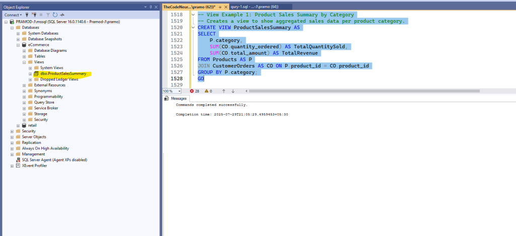
1. Product Sales Summary by Category
Let’s create a view that summarizes the total sales amount and quantity ordered for each product category.
-- View Example 1: Product Sales Summary by Category
-- Creates a view to show aggregated sales data per product category.
CREATE VIEW ProductSalesSummary AS
SELECT
    P.category,
    SUM(CO.quantity_ordered) AS TotalQuantitySold,
    SUM(CO.total_amount) AS TotalRevenue
FROM Products AS P
JOIN CustomerOrders AS CO ON P.product_id = CO.product_id
GROUP BY P.category;
GOOnce executed, you can see the new view you just created –
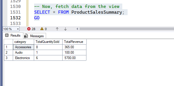
Let’s query the view –
-- Now, fetch data from the view
SELECT * FROM ProductSalesSummary;
GOOutput:
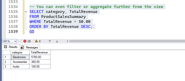
Check this query for how you can do further operations on the view –
-- You can even filter or aggregate further from the view
SELECT category, TotalRevenue
FROM ProductSalesSummary
WHERE TotalRevenue > 50.00
ORDER BY TotalRevenue DESC;
GOOutput:
The ProductSalesSummary view provides a pre-aggregated summary of sales by category. This view simplifies reporting on category performance without needing to perform the join and aggregation every time.
2. Detailed Customer Order Information
Often, you need to combine data from multiple related tables. A view can pre-join these tables, making subsequent queries much simpler.
-- View Example 2: Detailed Customer Order Information
-- Creates a view that joins Products and CustomerOrders tables.
-- This view provides a consolidated look at customer orders including product details.
CREATE VIEW DetailedCustomerOrders AS
SELECT
    CO.order_id,
    CO.customer_name,
    CO.order_date,
    P.product_name,
    P.category,
    P.unit_price,
    CO.quantity_ordered,
    CO.total_amount
FROM CustomerOrders AS CO
JOIN Products AS P ON CO.product_id = P.product_id;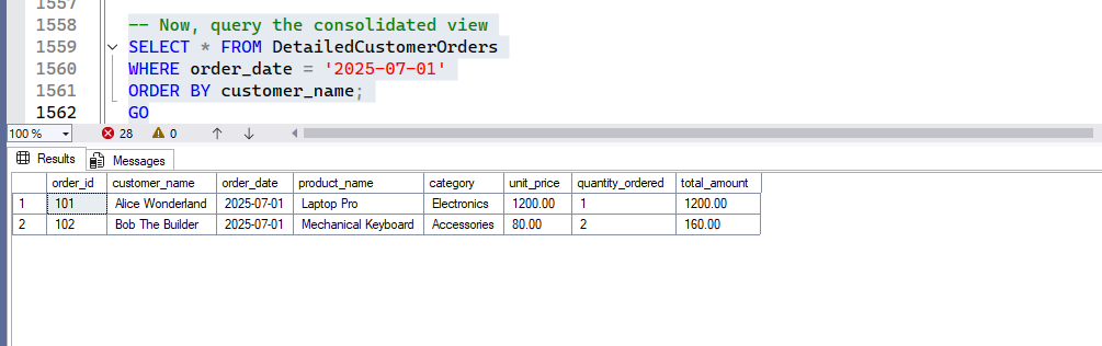
GOOnce executed, run the below query to check the created view –
-- Now, query the consolidated view
SELECT * FROM DetailedCustomerOrders
WHERE order_date = '2025-07-01'
ORDER BY customer_name;
GOOutput:
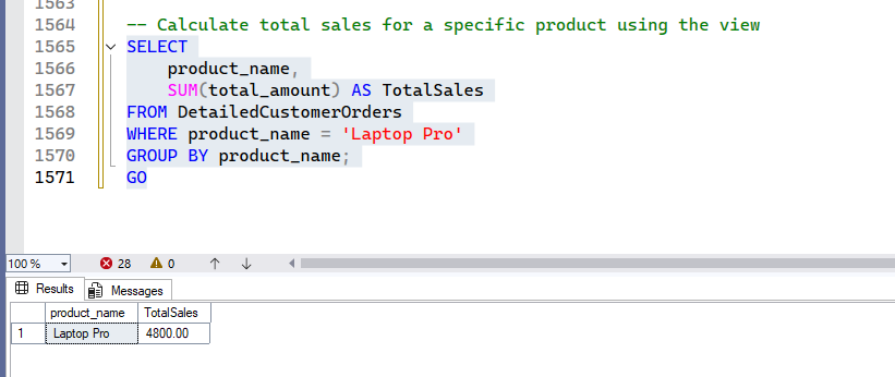
Now, calculate total sales for a specific product using the view –
SELECT
    product_name,
    SUM(total_amount) AS TotalSales
FROM DetailedCustomerOrders
WHERE product_name = 'Laptop Pro'
GROUP BY product_name;
GOOutput:
The DetailedCustomerOrders view acts as a single, wide table containing all relevant order and product details. This eliminates the need to write complex joins repeatedly, simplifying reporting and analysis for customer orders.
Ranking Window Functions: Ordering Your Data
Now, let’s dive deeper into a specific and very common type of Window Function: Ranking Window Functions. These functions assign a rank to each row within a partition of a result set, based on a specified ordering. They are indispensable when you need to find top N items, identify duplicates, or analyze data based on its position within a group.
The key to ranking functions is the OVER() clause, which defines the “window” of rows the function operates on. ORDER BY within OVER() specifies the ranking criteria.
1. RANK()
RANK() assigns a unique rank to each distinct row within its partition. If two or more rows have the same value for the ordering column, they receive the same rank, and the next rank in the sequence is skipped.
-- Ranking Example 1: Using RANK() for Student Scores
-- Ranks students within each subject based on their score.
SELECT
    student_id,
    student_name,
    subject,
    score,
    RANK() OVER (PARTITION BY subject ORDER BY score DESC) AS SubjectRank
FROM StudentScores
ORDER BY subject, SubjectRank;
GO
Output:
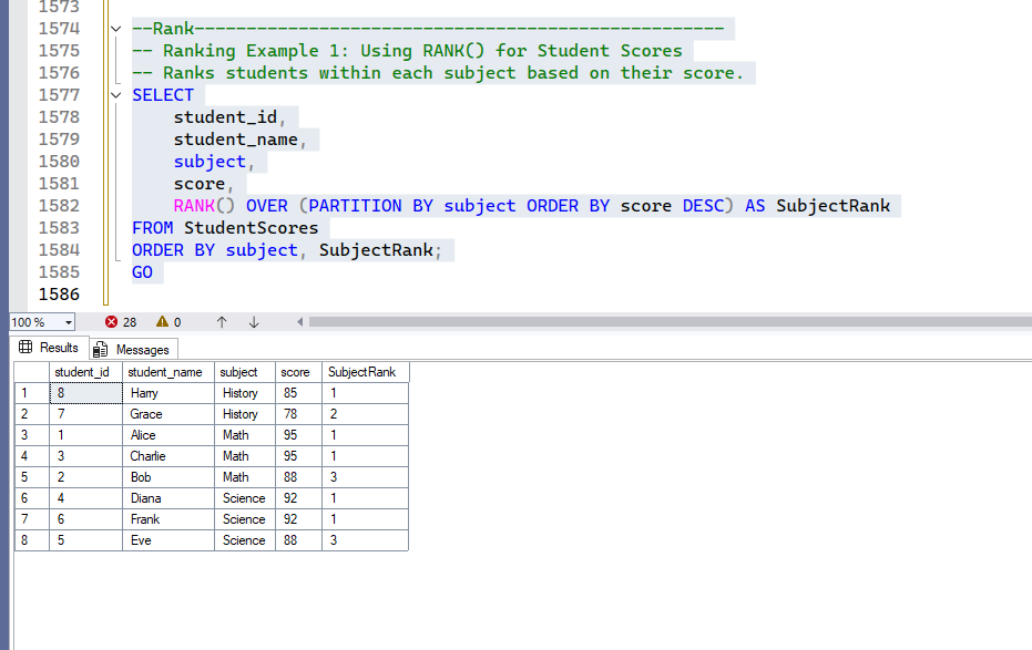
Explanation: ‘Alice’ and ‘Charlie’ both scored 95 in Math, so they both get rank 1. The next rank assigned is 3, skipping 2. Similarly for ‘Diana’ and ‘Frank’ in Science.
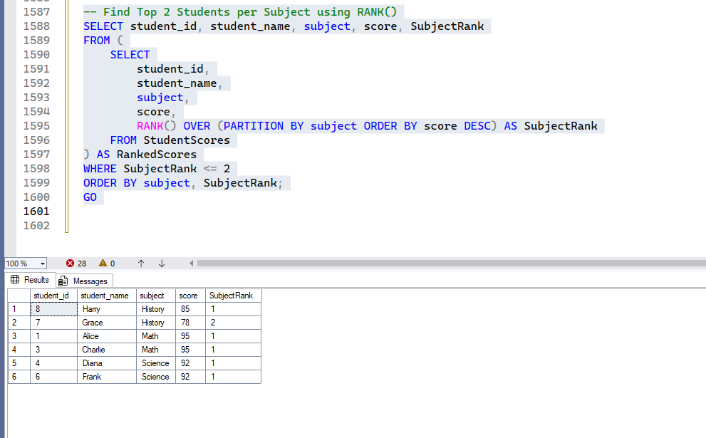
You can use this to find specific ranks, for example, the top 2 students in each subject:
-- Find Top 2 Students per Subject using RANK()
SELECT student_id, student_name, subject, score, SubjectRank
FROM (
    SELECT
        student_id,
        student_name,
        subject,
        score,
        RANK() OVER (PARTITION BY subject ORDER BY score DESC) AS SubjectRank
    FROM StudentScores
) AS RankedScores
WHERE SubjectRank <= 2
ORDER BY subject, SubjectRank;
GO
Output:
2. DENSE_RANK()
DENSE_RANK() is similar to RANK() but does not skip ranks in the event of ties. If two or more rows have the same value, they receive the same rank, and the next rank assigned is consecutive.
-- Ranking Example 2: Using DENSE_RANK() for Athlete Performance
-- Ranks athletes within each event based on their time (lower time is better).
SELECT
    athlete_id,
    athlete_name,
    event_name,
    time_in_seconds,
    DENSE_RANK() OVER (PARTITION BY event_name ORDER BY time_in_seconds ASC) AS EventDenseRank
FROM AthletePerformance
ORDER BY event_name, EventDenseRank;
GOOutput:
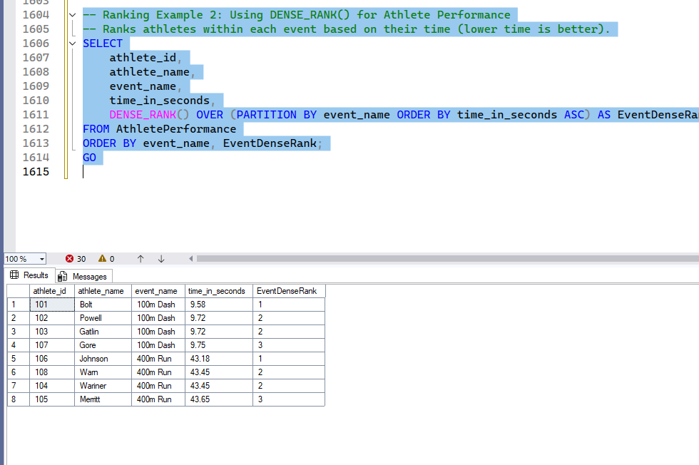
Explanation: Here, you can see there are 1, 2, 2, rank and still, 3rd rank, not 4th like Rank() as above.
3. ROW_NUMBER()
ROW_NUMBER() assigns a unique, sequential integer to each row within its partition, starting from 1. If there are ties in the ordering column, ROW_NUMBER() assigns arbitrary but unique numbers to the tied rows.
-- Ranking Example 3: Using ROW_NUMBER() for Unique Ordering
-- Assigns a unique row number to each student within their subject, ordered by score.
SELECT
    ROW_NUMBER() OVER(PARTITION BY subject ORDER BY score DESC) AS Row_num,
    student_id,
    student_name,
    subject,
    score
FROM StudentScores
ORDER BY subject, Row_num;
GOOutput:
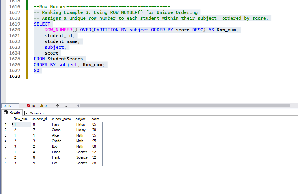
Explanation: ROW_NUMBER() is useful when you need a distinct sequential number for every row, regardless of ties. For example, if ‘Alice’ and ‘Charlie’ both have a score of 95 in Math, ROW_NUMBER() will arbitrarily assign one of them 1 and the other 2 within the Math partition. This is often used for pagination or when you need to select only one arbitrary row from a set of duplicates (e.g., the first entry for each student).
ROLLUP Function: Summarizing Your Data Hierarchically
The ROLLUP operator is an extension to the GROUP BY clause that generates subtotals for combinations of grouping columns, as well as a grand total. It’s incredibly useful for creating summary reports that show aggregates at different levels of granularity.
Understanding the IDENTITY Constraint: Auto-Incrementing Primary Keys
Before diving into ROLLUP, let’s take a moment to understand a new concept introduced in our EMPLOYEE table: the IDENTITY constraint.
CREATE TABLE EMPLOYEE (
    emp_id INT IDENTITY (1,1) PRIMARY KEY, -- IDENTITY (seed, increment)
    fullname VARCHAR(65),
    occupation VARCHAR(45),
    gender VARCHAR(30),
    salary INT,
    country VARCHAR(55)
);
The IDENTITY constraint is a powerful feature in SQL Server that automatically generates sequential numeric values for a column when new rows are inserted into a table. It’s most commonly used for creating auto-incrementing primary keys, ensuring that each new record gets a unique identifier without manual intervention.
Let’s break down IDENTITY (1,1):
1(Seed Value): This is the starting value for the identity column. The first row inserted will haveemp_id = 1.1(Increment Value): This is the value by which the identity column will increase for each subsequent row. So, the second row will haveemp_id = 2, the thirdemp_id = 3, and so on.
Why is IDENTITY useful?
- Uniqueness: It guarantees that each new row will have a unique
emp_id, which is crucial for primary keys. - Simplicity: You don’t need to manually manage or generate IDs for new records; the database handles it automatically.
- Data Integrity: It helps maintain data integrity by preventing duplicate or missing primary key values.
This is a very common and efficient way to manage primary keys in many database systems.
ROLLUP in Action
1. Simple ROLLUP (Single Column)
Let’s calculate the total salary per country, and then add a grand total for all countries.
-- ROLLUP Example 1: Total Salary by Country with Grand Total
-- Standard aggregation for comparison
SELECT country, SUM(salary) AS "Total Salary"
FROM EMPLOYEE
GROUP BY country;
GO

-- Using ROLLUP to add a grand total
SELECT country, SUM(salary) AS "Total Salary"
FROM EMPLOYEE
GROUP BY ROLLUP (country);
GO
-- OR (alternative syntax)
SELECT country, SUM(salary) AS "Total Salary"
FROM EMPLOYEE
GROUP BY country WITH ROLLUP;
GO
Output:
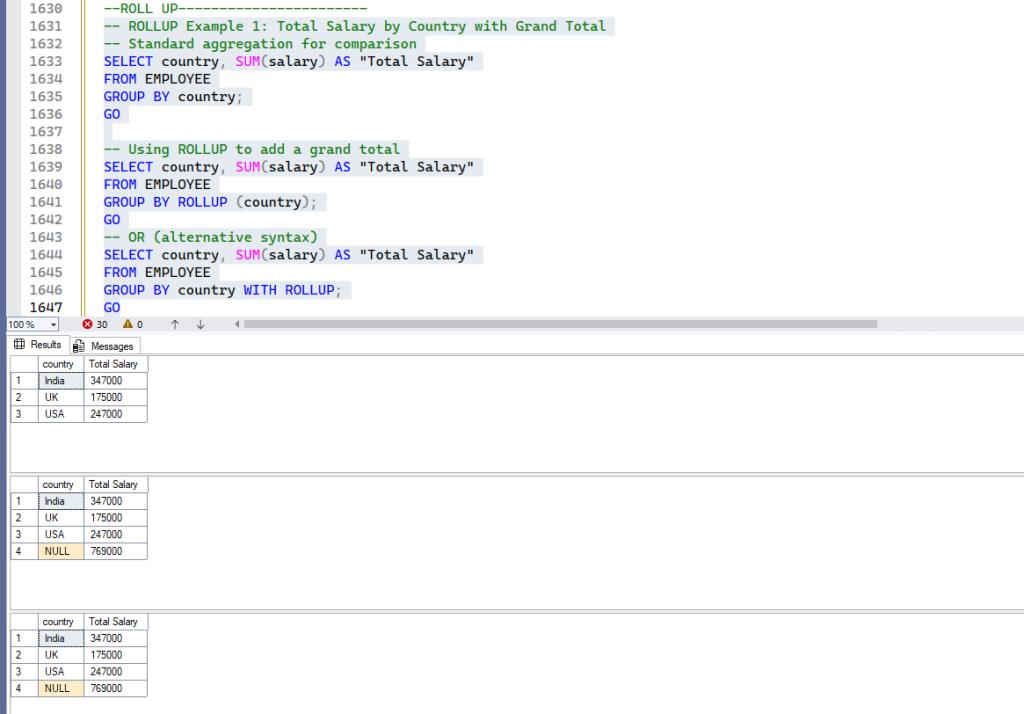
Explanation: The ROLLUP operator adds an extra row with NULL in the country column, representing the grand total of salaries across all countries. The NULL indicates the aggregation is at a higher level (the total for all countries).
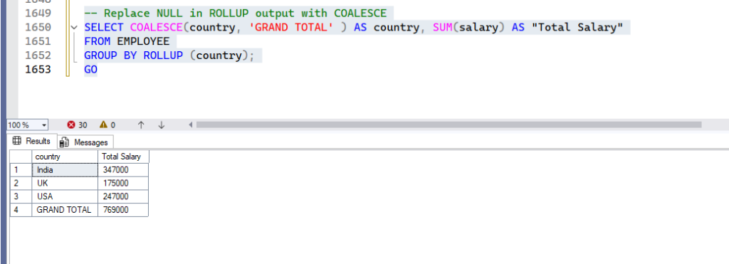
To make the NULL more descriptive, you can use COALESCE():
-- Replace NULL in ROLLUP output with COALESCE
SELECT COALESCE(country, 'GRAND TOTAL' ) AS country, SUM(salary) AS "Total Salary"
FROM EMPLOYEE
GROUP BY ROLLUP (country);
GOOutput:
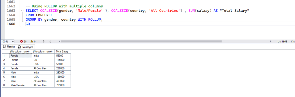
2. ROLLUP with Multiple Columns (Hierarchical Aggregation)
When you use ROLLUP with multiple columns, it generates subtotals for each combination of the specified columns, following a hierarchy. For ROLLUP (col1, col2), it will generate:
- Subtotals for
(col1, col2) - Subtotals for
(col1) - A grand total
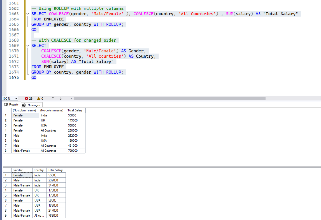
-- Using ROLLUP with multiple columns
SELECT COALESCE(gender, 'Male/Female' ), COALESCE(country, 'All Countries') , SUM(salary) AS "Total Salary"
FROM EMPLOYEE
GROUP BY gender, country WITH ROLLUP;
GOOutput:
If you change the order of columns in ROLLUP, the hierarchy of subtotals changes:
-- With COALESCE for changed order
SELECT
    COALESCE(gender, 'Male/Female') AS Gender,
    COALESCE(country, 'All countries') AS Country,
    SUM(salary) AS "Total Salary"
FROM EMPLOYEE
GROUP BY country, gender WITH ROLLUP;
GOOutput: To get more visibility, try running both the queries in one go to observe the output, how it was different for “GROUP BY gender, country WITH ROLLUP” vs “GROUP BY country, gender WITH ROLLUP;”
Conclusion
By mastering Views, you can create simplified, secure, and consistent interfaces to your database, abstracting away complex underlying structures. Ranking Window Functions (RANK(), DENSE_RANK(), ROW_NUMBER()) provide powerful ways to order and categorize your data, enabling you to identify top performers, manage duplicates, and analyze positional data with ease. Finally, the ROLLUP operator is an invaluable tool for generating hierarchical summary reports, providing subtotals at various levels of aggregation, culminating in a grand total.
These features, when used effectively, significantly enhance your ability to manage, analyze, and present data in MSSQL, making your queries more efficient and your reports more insightful.
Stay tuned for more!
Leave a Reply
You must be logged in to post a comment.